
Die Inhalte dieser Seite sind leider nicht auf Deutsch verfügbar.
Seitenpfad:
- Startseite
- Christian Hilgenfeldt
- A modified Version of the 2G Cryogenic Magnetometer
A modified Version of the 2G Cryogenic Magnetometer

T. Frederichs, C. Hilgenfeldt & K. Fabian
(abstract of poster presented at GFZ Potsdam, Germany, autumn 2000)
Since the 2G long core magnetometer 755 was installed in summer 1997 at the University of Bremen, various modifi- cations were made concerning technical and practical operations as well as the graphical user interface.
In addition to the conventional setup consisting of three DC-squids and three alternating field coils for demagnetization, the Bremen instrument is equipped with an internal pulse magnetizer (maximum field 800 mT) and a DC coil to generate anhysteretic remanent magnetizations in fields of up to 0.4 mT. To increase the system’s efficiency we developed a robot that automatically loads and unloads the magnetometer with sets of about 100 samples.
The integration of all these components provides the opportunity of applying the whole set of isothermal remanence measurements to discrete samples as well as to long-cores. Lining up several types of paleo- and rock magnetic measurements in combination with the use of the automated sample loader makes it possible to operate the magnetometer for several hours without intervention of the operator. Despite its uncontradicted benefit, the requests to the reliability of an automated system are more strictly than to those of a manually operated instrument. The mechanical and electrical/electronic stability is of the same importance as the user’s information about the measurement progress, the system status and last but not least about the data quality already during measurement.
After one year of operation we made modifications in numerous details attributed to the following major problems of the original setup:
- no temperature monitoring of the alternating field coils (high temperatures may severely damage the coils)
- no verification whether desired alternating field values have actually been reached (magnetization curves may be erroneous)
- no monitoring of the sample holder position (may lead to damage or inaccurate magnetization curves)
- inconvenient data display (no opportunity to assess the data quality in order to terminate a sometimes not repeatable measurement)
In consequence we implemented the following features:
- thermocouples on AF coil surfaces (software waits for the coils to cool before measurement continuation)
- controlled software shutdown if desired field value has not been reached or the sample holder position was not correctly determined
- display of all data of all samples during measurement (Zijderveld graphs, magnetization curves, etc.)

The above mentioned modifications were carried out by developing a completely new LabView-based software (Fig. 1) including the following options:
- second PC which operates for safety reasons since the installation of the automated sample loader, because robot and magnetometer are two completely separated systems, which should react in a convenient way to malfunctions of their counterparts
- connection between both PCs, to the local area network and the internet, therefore monitoring is possible not only locally in the laboratory but also from every connected PC
- information of the operator at office PC or via pager or mobile telephone at the end of the measurement cycle or in case of a system shutdown
- generating of script files for use of the automated sample loader to process any type of measurement (demagnetization, ARM & IRM acquisition) for different sample sets
- Transparency of data acquisition and processing is a fundamental request of scientists to evaluate data reliability. Considering this the measurement data are processed in the following way:
- raw data storing immediately after acquisition and transformation into a suitable format at the end of a measurement cycle
- storing in separate files for each step of data manipulation
- documentation of the complete program course in log files with (nearly) all parameters for debugging or subsequent control
Beside the improvements concerning data acquisition we modified also the procedures of IRM and ARM acquisition:
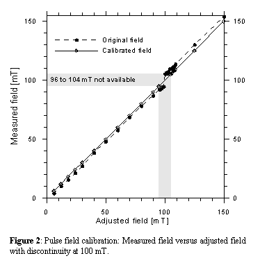
IRM acquisition experiments show that the magnetic fields generated by the internal pulse magnetizer do not increase linearly from zero to maximum. Measurement of the effective field strength proves a gap between nominal 99 and 100 mT. Lower fields are relatively too small, higher fields too large. Therefore we integrated a calibration function in the software, that corrects for this effect. Due to the discontinuity at fields around 100 mT, real fields between 95 and 105 mT are not available (Fig. 2).
IRM acquisition experiments show that the magnetic fields generated by the internal pulse magnetizer do not increase linearly from zero to maximum. Measurement of the effective field strength proves a gap between nominal 99 and 100 mT. Lower fields are relatively too small, higher fields too large. Therefore we integrated a calibration function in the software, that corrects for this effect. Due to the discontinuity at fields around 100 mT, real fields between 95 and 105 mT are not available (Fig. 2).
The ARM acquired by the ‘dynamic’ process implemented in the original software was often found inconsistent with an ARM generated by the classical stationary method. The shape of the ARM acquisition curve was inaccurate and the maximum remanence was distinctly reduced. These dissimilarities were caused by the remanence acquisition process: The original software moves the sample with a certain velocity through the coils after they had reached the desired field value. The field is kept constant until the complete sample holder has moved through the coils. The increasing and decreasing field intensity is achieved by means of the axial distance of the sample to the coils. Critical for the acquired remanence is the velocity used to move the samples through the coils. Depending on the sample’s magnetic properties we found differences in intensity of up to 40% (Fig. 3).
To avoid these problems in the new software, we returned to the classical/stationary ARM acquisition process. The alternating field increases after the sample is placed in the center of the coil and decreases when the desired maximum field was reached. The sample remains in the coil center during the entire process. Afterwards the next sample is treated in the same way. This procedure slows down the measurement progress but is necessary to ensure comparable data sets.
To avoid these problems in the new software, we returned to the classical/stationary ARM acquisition process. The alternating field increases after the sample is placed in the center of the coil and decreases when the desired maximum field was reached. The sample remains in the coil center during the entire process. Afterwards the next sample is treated in the same way. This procedure slows down the measurement progress but is necessary to ensure comparable data sets.
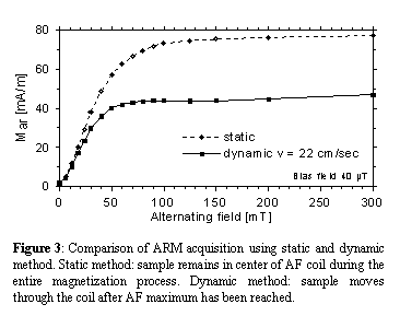
From a theoretical point of view it can be shown that the loss of intensity by the ‘dynamic’ method is proportional to the difference DH of two subsequent half cycles of the alternating field. DH is minimal for a static sample and increases with increasing velocity of the sample.