
Digital imaging
Please find the details for operating the digital imaging systems to the right.
Digital imaging (on superslit XRF scanner)
The color line scan camera is a 3 CCD device using 3 x 2048 pixel CCD arrays and a beam-splitter. The linescan software produces visual color images (BMP, TIF and JPG) but also color data in RGB and CIE-L*,a*,b*.
Important information:
• Camera and the light of camera should be allowed to warm up for at least one hour before calibrating or collecting images.
• When the optic unit is moving: please stay away from the scanner!
1. Switch on the XRF Core Scanner (XRF3) for line scan images
• Turn the main switch (big red switch) a quarter to the right.
• Please wait about a minute until the scanner is ready (can be observed in the touch screen). Press the blue “reset emergency button” and press on the touch screen “reset error” and “reset cycle”. Open the scanner door.
• Press the „Light Camera“ – button and wait at least 1 hour (!!) before you can start the line scan.
2. Camera Set Up (Calibration)
The main Set Up procedures to calibrate the camera are: black/white calibration, set ting the aperture and adjusting the focus. We advise to keep the aperture and the focus fixed for the entire core to be imaged.
2.1. Getting started
• Switch on PC and monitor.
• Click on the program icon „Camera V1.8 “.
• Connect PC to scanner by clicking on the tree icon.
2.2. Black/White calibration
White calibration is performed with the white calibration tile. The camera moves to the tile; please make sure beforehand no dust is on the tile. Black Calibration is performed with the cap on the lens.
• White calibration: For calibration use aperture 11+ first and remove cap from lens. Click on “white calibration scan” in the pull down menu and hit “play”: white calibration is performed now. The RGB data in the histogram should be on the right side of the histogram. A white calibration file is created that corrects the image data to a known white standard.
• Black calibration: put the cap over the lens. Choose „black calibration scan“ in the pull down menu. The RGB data should be on the left side of the histogram. Attention: Remember to remove the cap!
2.3. Set Aperture
• Wait until the entire core to be imaged is split and ready.
• To set the aperture place the section with the lightest part of the core under the camera and adjust the aperture using the quick scan option in the pull down menu such as red, green and blue show high intensity values on the right side of the histogram. If pixels are over-exposed peaks reach over 255. Select the appropriate aperture setting in the measurement setup box in the „Camera V1.8 “application.
2.4. Set Focus
The focus is already set by the technician. In case it should be corrected please place the striped card on top of the section surface (position 1000 mm).
• Click on „focus scan“ in the pull down menu. The optic complex will move to this point and you can observe the focus scan on the monitor.
• For adjusting the focus use the lower ring of the camera objective while you observe the monitor. Note: there is a small delay between adjusting the focus ring and the resulting changes displayed on the monitor.
• To end the focus scan click on “stop”. Attention: the optic complex is moving to the initial position. Stay away from the scanner.
3. Acquire, Edit and Upload Image
3.1. Acquire Image
3.1.1. Section preparation
• The surface of the sediment should be as smooth as possible, please prepare adequately with the tools. Do not cover the sediment with foil!
• Measure the length of the section in cm.
• Place section correctly in the holder: top must be at 0-point of the ruler.
3.1.2. Quick Scan
• Click on „quick scan“: a quick line scan is performed. Please observe the histogram. All RGB data should be in the histogram. If the curves cannot be completely found in the histogram, please adjust the aperture and do the „quick scan“ again.
Note: Do not change the aperture setting while acquiring images from a core (multiple sections).
3.1.3. Line Scan
• Select measurement setup in Setup and fill in the following:
Sample name:325_M0042_A_003_R_01_scan
Sample length:Length in cm (no decimals behind the comma!!)
max. length = 154 cm!
Lens aperture:value at camera objective
Save image as:click on BMP and JPG
Save color data as:click on TXT
Change directory:OSP_New Jersey_line scan\28A\28A-3R
• The RGB and CieLab data are automatically generated and saved in the .txt-file (section folder). The area is between 750 and 1000 pixel.
Note: After each core the gray and the color reference chart must be scanned (e.g. place charts after core catcher).
After the image of a section has been taken, please check quality and cut off all pixel of the .bmp-image outside section and gauge.
• Open image .bmp in adobe photoshop.
• With cut tool edit image.
• Copy image (ctrl c).
• Open new file (ctrl n) and paste image (ctrl v).
• Save the cut image under the proper folder naming 325_M0042_A_003_R_01_scancut
• In the panel “bmp options” click ok.
• Close both images.
3.3. Upload to server
•Click on “My Computer”, “Science_Folder_NJ on Network Attached Storage (10.1.8.9) (N:)”
• Password: rcb.
• OSP_Science_Folder.
• Line_scan_images.
• Now copy the entire folder of the core imaged into the Line_scan_images folder.
3.4. Data file/meta data
In the automatically generated and saved .txt file (in the folder of each section) you will find the RGB data and l*a*b* data in 66 µm resolution as well as the following meta data:
Down Core (ppcm)
Cross Core (ppcm)
First Pixel_DC
Pixel Count_DC
First Pixel_CC
Last Pixel_CC
White Calibration Level
Aperture
4. Switch off scanner
• Remove any section from scanner.
• Switch off the light and close scanner door.
• Turn main switch a quarter turn to the left.
• Shut down the PC and monitor.
• Close all Lab windows and lock the Lab by key.
5. Trouble shooting
1.If the error message “file not found” appears when you click on the 3rd icon from the left, please:
• close the program
• go to C:\\program files\WinLinescan\WinLinScan1.8
• delete SetupSample.cfg file
• Open the „Camera V1.8“ software again: a panel with “ Restoring default Measurement Setup” appears. Click ok.
• Perform only the White Calibration again (aperture 11+)
2.If camera is not working or not working properly: check cable connection on top of camera.
3.If image looks too dark although the right aperture is used: check if lamp is ok.
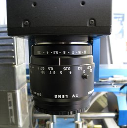
The camera objective of the optic unit: the upper ring shows the aperture, the lower ring the focus.
Digital Imaging (Geoscan III on MSCL)
Soon after splitting of the core the archive half is scanned by a CCD, which is mounted on the rack of the Multi-Sensor Core Logger. Please find below the details for operating the digital imaging system.
The GEOSCAN colour line scan camera is a 3 CCD device using 3 * 1024 pixel CCD arrays.
Light from the object passes through the lens and is split into 3 paths by the beam splitter to fall on the red, green and blue detectors (RGB), which when combined reproduce a conventional colour image.
Main menu
Right after switching on camera and light source, Set Up must be performed before acquiring images. It takes 30 to 45 minutes including a test image.
Within most of the set up screens both a RGB Scope and the Camera Control Panel will be displayed. The RGB Scope got different display options.
The Camera Control Panel allows the operator to move the pusher within the software by either dragging the pusher to the desired location or using the nudge arrows provided.
The main Set Up procedures are:
- Black and White Calibration
White Calibration is performed with the white calibration tile. The camera travels a short distance across the tile to remove the effects of any dust on the tile. Choose the Camera Control Panel to first set a reference point and nudge the pusher so that the white tile is in the position needed for calibration (3 x 90% must be checked for the white calibration. Alternatively you can use the gray calibration tile (3 x 18 % must be checked in the Control Panel)).Follow the instructions on the screen. A white calibration file is created that corrects the image data to a known white standard. The camera looks PC-controlled for the best aperture.Black Calibration is performed with the cap on the lens. Do not forget to remove the cap after calibration!. Follow the instructions on the screen.


- Set Aperture
The aperture of the lens should be set so that the entire core can be imaged with the same setting. Therefore the lightest part of the core should be placed under the camera and the aperture adjusted via PC such that the red, green and blue responses from the CCDs do not saturate. The camera looks PC-controlled for the best aperture.In case it is necessary to optimize the aperture, the operator should select the appropriate aperture setting in the ‘Control Panel’. The camera will then be adjusted to the chosen aperture.

- Set Focus
Place a sharp black to white boundary (e.g. focus bars on test card) under the camera at the level of the core surface. When clicking “auto” in the ‘Control Panel’ wait until the lens of the camera has found the best focus. The focus bar should show the maximum value possible.

- Camera Utility
The Camera Utility Panel provides access to the actual RGB Scope and the Camera Control Panel. - Horizontal Resolution
The Horizontal or Cross Core Resolution is controlled by the lens and the height of the camera above the object. It only has to be changed when the height of the camera or the lens is changed. It is limited to 1000 pixels wide.
To define the cross-core resolution the user must place a subject with blocks of black and white (of known width) under the camera at the level of the core surface. The user must then move the marker lines over the edges of the known width and enter the known width into the text box at the top left of the scope. - Cross Core Convergence
The mechanical configuration of the CCDs within the camera head is set at the time of manufacture and the convergence values (alignment errors) are setup when the camera is installed. However, if the camera is subjected to mechanical shock then the alignment of the CCD sensors should be checked. - Crop Points
This option allows the user to discard data at the edge of the CCD array, for example if a particular cross-core resolution is required then this may leave parts of the image without any useful data in. The data that is not recorded to file is simply saved as black pixels. - Change Resolutions The down-core resolution is controlled by the line acquisition rate as synchronised to the stepper motor. The base resolution should always be set to 25µm/400 ppcms (do not change the base resolution! The visible resolution can be set to 100 µm/100 ppcms or to the standard visible resolution 50 µm/200 ppcms.

- Acquire Image
In the Camera Control Panel the user enters the core sections to be logged. Sections can be added [New], deleted [Delete] and attributes can be changed [Edit] at any time during the imaging process.

When editing a core section, the acquisition panel shows up.

Create your own directory under
D:\Geotek Data\XXX
Set the reference position of the pusher (step motor) by zeroing the pusher in the ‘Control Panel’. The motor must be set to “auto”. When the pusher is at the right end/side, click [Move Nominal Position] and the pusher moves back the nominal section length. Adjust the first section to be scanned on the track that the bottom of the section is touching the pusher.
Click [Begin Scan] to start scanning the first section. The pusher will automatically look for the reference point to start scan.
After each section the pusher will move back the nominal section length and ask you to continue scanning.
Each section is saved as tiff-file with app size per 1.5 m scanned:
100 ppcms: ~ 104.011 KB
200 ppcms: ~ 415.866 KB


- Extraction of Red, Green, Blue (RGB) data
Open the software “Image Tools” on the desktop. Select your line scan image. Define the interval of interest (usually an interval of 1 cm in the middle of the section) and click on “RGB analysis”. A small panel appears. You can choose your resolution down core, e.g. 0.1 cm. Click on “Create RGB files”.The RGB file is saved in an export folder. Open the file in Excel and check your data.IN case you want to change the wettings (e.g. width, interval) of the RGB data, got to the the software "Image Tools 3" on the desktop. Open the program, your line scan image, and click on" RGB analyses" (left).Now you can adjust the RGB data area width and interval. Rename your output file extension: xxxx.rgb. Click on "Create RGB files" and the new RGB file is saved in the export folder.


- File format and "ruler"
Click on “Export images” (right) and click on “create an image with a ruler using the settings”. Choose the appropriate format for your file: jpeg, tiff, png, bmp. If necessary compress the file format. You will be asked, where to save your data. Choose your folder and ceck your image with the ruler.


