Multi-sensor core logger (MSCL)

MSCL at MARUM, University of Bremen, with all sensors

The Multi-Sensor Core Logger (MSCL) measures the attenuation of gamma rays (gamma ray attenuation, GRA), the velocity of compressional waves (P-wave velocities), and the amount of magnetically susceptible material present in the sediment as well as the color reflectance by the spectrophotometer. The cores are transported by the pusher system. Split cores or whole rounds of up to 150 cm in length and from 6 to 15 cm in diameter can be used.

Preparation

Bring the cores to the lab several hours in advance to allow equilibration to room temperature (= constant), magnetic susceptibilities and P-wave velocities are temperature-dependent.

Cover split cores with foil as indicated. For good contact of the P-wave- transducers moisten the foil on the sediment with a thin film of distilled water, but do not soak neither the core nor the transducer! Please take care to not get water into the lower transducer!

A short handling instruction is available below, where you find some recommendations you should consider before you start core logging.

Keypoints-before-core-logging.pdf (15.6 kB)

Measurement

Starting

start the computer
put the 2 main switches on the electronic rack on (from bottom)
for line scan: put all 3 main switches on

Choose [Log New Core]
The following Panel will appear:

Create your own folder under D:\geotek\___ choose this directory in the File Panel and enter a Filename (e.g. name of the core). Click [OK] when ready.
The Configuration Panel will appear.

start computer
put the main switch on the electronic rack on
push power button at the oscilloscope (central unit)
turn rotary switch at suceptibility meter (uppermost unit) to "SI"
put switch of interface box on the back of the rack to 1
flip switch at the transformer box on ("1" )

Select the sensors.
For the processing you also need to acquire the Core Diameter.

For Gamma Attenuation choose at least 5 sec. count time, for the calibration choose 10 sec count time.
For Magnetic Susceptibility choose 3 sec. count time and SI unit.
See relating pages for further information on the different sensors (especially calibration notes!).

At the track
If you need the core diameter put reference core between the transducers.
Choose “Acoustic” motor and "Manual" and follow the instructions in the Logger Control Panel (PC).
Important: switch the track to “Auto” right after you set the reference core thickness!
Vertical Excursion should be between 25 to 40mm.

For setting the reference point choose “Pusher” motor and “Manual” and follow the instructions in the Logger Control Panel (PC).
Choose the Blue Tape Arrow at the track as Reference Point.
Choose “Auto” as soon as you set the reference point, put the first section on the track and adjust the pusher so that the top end of the core section is at the reference point.
Check that pusher is at block by trying to push it back!

During Measurement
For aborting a log you have to first click “Pause”, then “Abort”. All data measured till that point will be saved.
After finishing the first section the pusher moves to the end of the nominal section length. Put second section on the tracking system, move pusher to the end of this section and click "Continue". The configuration Panel will appear again. Check for the sensors you want to use (especially count time).

After a section went through all sensors it must be removed from the track. Otherwise the section will drop on the floor!

For finishing logging you have to log a dummy section of the length of the offset from the reference point to the last sensor you are taking measurements with. (offset magnetic susceptibility_loop sensor = 85cm, offset magnetic susceptibility_point sensor = 51cm, Spectrophotometer = 61cm, gamma density = 21cm, p-wave and core thickness = 39cm).
For the dummy section you can disable all sensors.

Graphical Data display
Raw data
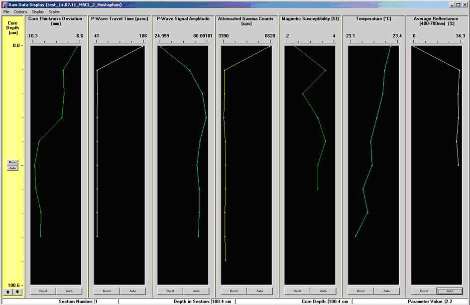
After the first measurement point of the first sensor the raw data display will appear.

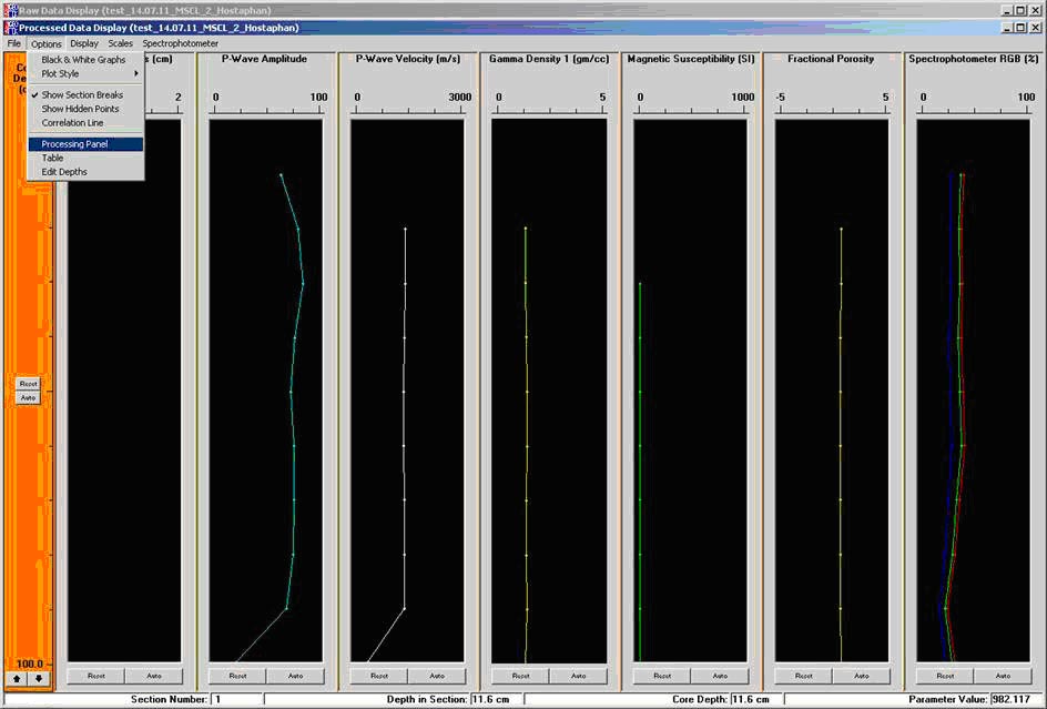
You can change axis by clicking on [Reset][Auto] or enter limiting values by choosing one of the axis.

After the whole core is logged the data must be processed.
Choose "Process Data" under "Options" in the "Raw data display ", the "Processed Data Display" will be opened.

Choose “Processing Panel” under “Options” in the “Processed Data Display” and the “Processing Panel Display” will be opened.
For each measured parameter you have to fill in the values according to calibration (see individual sensors for details).
The processed data is calculated from the raw data and calibration parameters according to pre-defined equations. The user can select (or deselect) which parameters are to be processed simply by clicking on the parameter of interest.

Initially (as raw data is collected) the sub bottom depth is calculated assuming that the top of section 1 has a sub bottom depth of zero. All other sub bottom depths are automatically calculated assuming that all other sections are sequentially logged and adjacent to each other. In the processed data the sub bottom depth can be recalculated by assigning a value to the top of section 1 (sub bottom depth offset) and by assigning a butt error distance. The butt error distance is the increase in length caused by the addition of end-caps that are normally placed around the end of the core liners on each section.

Choose “File” and “Create ascii” in the Processing and the Raw data Panel for saving the data as an ascii-file.

Temperature

A standard PRT (platinum resistance thermometer) probe is used to measure temperature. The probe is connected to a long flying lead that can be most conveniently inserted into the end of each core section as it is loaded onto the RH section. It is most important for accurate velocity measurements in sediments because velocity changes by approximately 3 ms per °C.

Magnetic susceptibility

For whole-round cores Bartington loop sensors MS2C, Ø: 80mm or 130mm are used. For split cores Bartington point sensor MS2E is installed.

The Magnetic Susceptibility sensor must be zeroed manually before measuring by pushing the knob at the Magnetic Susceptibility Panel (left hand at electronic rack) to the right. Let it count for a few seconds and put the knob back to initial position again.

For measurement the point sensor always has to touch the sediment surface but must not press into the sediment by force.

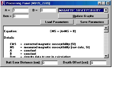
For processing you have to fill in the values A, B and Den.
A and B are constants (A = 1/ B = 0)
Den: density data to use in calculation:
Enter “0” if you do not wish to adjust for density
Enter “1” if you use gamma density 1

The instrument is preset to display the susceptibility values in volume or mass spefic SI or cgs units.

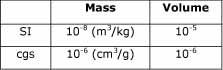
Magnetic susceptibility preset units

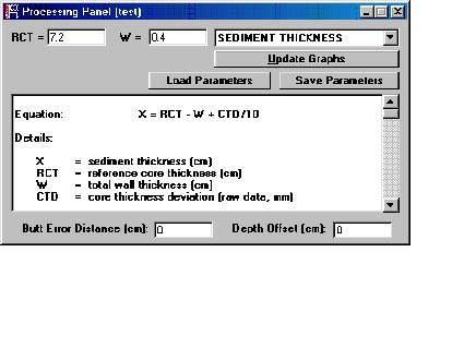
Sediment thickness

For processing the raw data the core diameter is important. Therefore it is important to measure a reference core thickness (RCT) of known diameter at the beginning of logging the core. The Logger measures then the deviation from the RCT (IODP-full 7.2 cm, IODP-half 3.6 cm, GeoB-full 12.5 cm, GeoB-half 6.25 cm).
In the processing Panel the RCT and the wall thickness of the liner has to be inserted in order to get absolute values.

GRAPE Density

Gamma Ray Attenuation Porosity Evaluator (GRAPE)
Open Gamma-Source:
- front position: 2.5 mm (standard)
- between the two stripes: 1 mm
- left beneath black tape: 5 mm

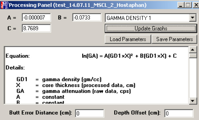
Calibration of gamma attenuation and calculation of densities
For each kind of liner a calibration must be performed and due to the decay of the gamma source (¹³⁷Cs, half life period of 30.4 years) at least once in 24h.
• take the count rates for the "telescope standard" for different diameters (count time at least 10 sec.!)
• calculate the mean for different countings and create a spread sheet with the following columns:
thickness of the calibration material (cm) / count rate (cps) / (thickness x density) / ln (count rate):
(see cal_Gamma.xlt)

Depth in standard (cm)	Thickness (cm)	Counts per second (cps)	Thickness x density (g/ccm)	ln cps
0	0	6436	0	8.769662508
8	1	5374	2.71	8.589327789
16	1.75	4605	4.7425	8.434897949
24	2.5	4007	6.775	8.295798111
32	3.25	3425	8.8075	8.138856751

Plot ln (cps) versus (thickness*density).
Calculate the gradient of the straight line (2nd derivation) (easiest by using a graph programme).

Use the resulting parameters (A, B, C) for the Processing Panel.

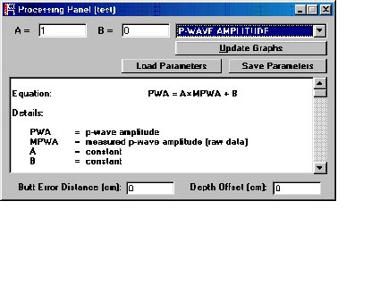
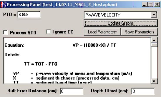
P-wave veolcity

Actually this calculation is only valid for "fry" sediments". For water saturated sediments a calibration would be needed where the Aluminium plates are in (sea)water.

For good contact of the P-wave- transducers moisten them and the foil with some dest. water, but do not soak neither the core nor the transducers. There must always be contact between sediment res. liner and transducers.

Calibration and Calculation of P-wave velocities
The propagation velocity of the ultrasonic pulse through the sediments inside the core liner is given by:

V = d/t (1)

d: diameter of the sediment core
t: pulse travel time in the sediment

The measured travel time (T) is given by:

T = t + (2)

all the additional time delays (caused by the liner, transducer surfaces, electronics).

The measured diameter (D) is given by:

D = d + 2w (3)

w: wall thickness of the core liner.

Therefore:

V = (D-2w)/(T-)

or

= T -((D-2w)/V) (4)

is the delay time needed to calibrate the system for a given liner and is input as the "P-wave travel time offset" (PTO).

• measure the core liner wall thickness,
• insert a liner filled with destilled water between the faces of the P-wave transducers, measure overall core diameter (D), overall travel time (T), and the temperature of the water.
• velocity (V) of the destilled water at a given temperature should be looked from a standard reference source (e.g.):

Temperature (°C)	Velocity (m/s)
0	1404
5	1435
13	1470
15	1477
18.5	1485
25	1509
35	1534

Calculation
Note that it is very important to compensate the measured sediment velocity for temperature. The temperature of each core section should be measured during logging and the velocity calculated for a specific temperature. If the measurements are around room temperature then the following approximation may suffice:

V20 = VT+ 3* (20-T)

V20 = velocity at 20°C
T = temperature
VT = velocity at the measured temperature T

Calibration example:

Parameter	Unit	Value	SI unit
Temperature of water	°C	21	21
Velocity of water	m/s	149	1495
Wallthickness	mm	3	0.003
Diameter of core	mm	70	0.7
Travel time	µs	50	0.00005
P-wave travel time offset	µs (s)	7.190635452	7.19064E^-06
Total diameter	mm	80	0.08
Total travel time	µs	48	0.000048
Velocity in sediment	m/s		1813.309294

P-WAVE TRAVEL OFFSET (PTO) for different liner:

ODP-Liner, wholeround 8.079 s
at:
temperature = 21°C; velocity in dest. water at this temperature = 1485 m/s; runtime = 88.25 s; diameter = 125 mm, wallthickness = 3 mm

ODP-Liner, halved 6.94 s
at:
temperature = 21°C; velocity in dest. water at this temperature = 1485 m/s; runtime = 51.85 s; diameter = 70 mm, wallthickness = 2.5 mm

Setting up signal levels:

Check that the transducers move freely in and out their housings against the spring pressure.
Position a water filled test core between the 2 PWT´s and adjust and tighten the position of each transducer housing such that a piston transducer are pushed approximately half way into their cylinder housings.
Wipe the core liner with a wet sponge and drop a little water onto the contacts between the transducer faces and core liner to provide a good acoustic coupling. Do not overwet, it does not help!
Oscilloscope: use "delay" as the negative trigger pulse, "signal" on channel 1 and "count" on channel 2. Set the delay thumb-wheel switch to 0 and set up the oscilloscope to clearly display the received signals. A large pulse should be clearly visible together with a number of equally spaced multiple arrivals on channel 1.
Increase the delay time by adjusting the thumb-wheel switch and adjust the time base on the oscilloscope until the direct pulse is expanded and clearly visible on the screen. The bar graph amplitude display should read >7 across a water core.
Check that the count pulse occurs at the zero crossing following the first negative excursion (see figure). If not, the "scale" and "offsets" adjustments for the threshold detector need resetting. Note that the threshold and zero crossing pulses can be monitored directly from the front panel.
Remove the water core and observe the transmission through air. Check that the count pulse occurs at the zero crossing following the 1st negative excursion (see diagram). If not "scale" and "offset" adjustments for the threshold detector need resetting.

"Pulse timing circuitry": The automated P-wave measuring system uses an easily identifiable zero crossing to measure the travel time of the pulse. The first negative excursion on the pulse is picked up by a threshold detector.
The transmitter pulse is sent to the transmitter transducer which generates an ultrasonic compressional pulse at about 500kHz. This pulse propagates through the core, is detected by the receiver, and is amplified by the AGC (Automatic Gain Control). A delay pulse is generated by the system after the transmit pulse has been sent. The delay time is set by the thumb-wheel switch and should be a few microseconds less than the travel time for the beginning of the received pulse. A gate pulse is generated (set by the thumb-wheel switch) after the set delay time, during which period a peak detector measures the amplitude of the incoming signal. A zero crossing detector detects all zero crossings and can be monitored through the "zero crossings" output. The count pulse, which is the signal required, is triggered as the 1st zero crossing after the threshold has been exceeded. In practice, it is necessary to check that the "count" pulse consistently aligns itself with the designated part of the received pulse.

Data processing

PTO = P-Wave Travel Time Offset

T = Temp °C
S = Salinity ppt
D = depth m
You can choose processing without STD!

Turn off

Make copies of your files and take them to floppies:
*.dat = raw data file
*.raw = raw data ascii-file
*.out = processed data ascii-file
Turn off the PC
Push power button at the oscilloscope
Power off at microprocessor unit (below right)
Switch interface box off
Close shutter of gamma source! Close the padlock!
Flip switch at the transformer box to "0".
Remove the plug from the socket.